Formula 1 popularity analytics using R
Here's what's been keeping me busy this summer - alongside of course, a truck load of movies and TV shows and books.
So we all know what Twitter is. The whole world is out there, and if you aren't yet, you should seriously consider joining.
Second, there's this remarkable statistical analysis tool which is called R. Read about it here. With Twitter, we have a lot of data to analyse, and with R we get the power to analyse all that data. Which is exactly what we're going to do.
So, get yourself a Twitter account, if you haven't already; install R Studio on your system (R Studio is a neat IDE that you can use to write programs in R), and let's proceed to do a pretty cool experiment.
What is our aim?
We're trying to analyse live tweets, to do a popularity analysis of two topics. Since I'm a motorsports buff, I'll choose two Formula 1 drivers as my guinea pigs (Sebastian Vettel and Kimi Raikkonen). You can choose anything you want, from Lady Gaga and Rihanna to Manchester United and Arsenal.
So roll up your sleeves and let's get started.
To use Twitter's APIs for R, we need to configure R and install some packages. Also, you'll be needing your own Twitter application which you can register and get for free at http://dev.twitter.com. Before that of course, you'll need a Twitter account.
Creating your Twitter App
So login to dev.twitter.com using your Twitter credentials. Go to My Applications > Create a new application. Fill in the required fields sensibly. You will then get a lot of data, two of which you need to save and keep handy. Your "Consumer Key" and your "Consumer Secret". Next, go to the Settings tab and set "Read, Write and Access"
Setting up R for use with Twitter
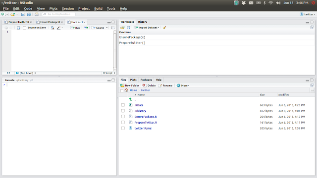
The package that you'll need to fetch and analyse Twitter data using R, is called TwitteR. (Yeah, seriously.) So start up R Studio. You'll be greeted with a screen similar to this.
Now go to Tools > Install packages and search for and install the following packages from the repositories. (Just start typing the name of each package and it'll show up in a drop down menu.)
bitops
RCurl
RJSONIO
twitteR
ROAuth
Once they've been installed, restart RStudio.
Next go to the bottom right frame of your workspace and click on the "Packages" tab. You'll see that the new package names have come in there. "Check" the new ones.
Now you need to verify your recently created application's credentials for use with R.
So key in the following code in the workspace prompt.
I terribly regret the fact that I couldn't copy paste the code here, because Blogger's retarded text editor parses every unusual symbol as HTML or XML or some form of styling. So wherever I was unable to write the code here, I decided to take screenshots of my console. Shoddy? Yes. Do I like it? No.

Yeah, this looks messy. But let's try to understand what we just did.
We created a new variable called credential using the in-built function OAuthFactory$new. We supply as parameters, our consumer key, our consumer secret and some parameter URLs which the function needs to test the credentials and verify the keys. Now credential is a data structure which has certain inbuilt functions in it. We'll need one of them to create a connection and verify its genuineness. Hence, type in the next piece of code.
So we all know what Twitter is. The whole world is out there, and if you aren't yet, you should seriously consider joining.
Second, there's this remarkable statistical analysis tool which is called R. Read about it here. With Twitter, we have a lot of data to analyse, and with R we get the power to analyse all that data. Which is exactly what we're going to do.
So, get yourself a Twitter account, if you haven't already; install R Studio on your system (R Studio is a neat IDE that you can use to write programs in R), and let's proceed to do a pretty cool experiment.
What is our aim?
We're trying to analyse live tweets, to do a popularity analysis of two topics. Since I'm a motorsports buff, I'll choose two Formula 1 drivers as my guinea pigs (Sebastian Vettel and Kimi Raikkonen). You can choose anything you want, from Lady Gaga and Rihanna to Manchester United and Arsenal.
So roll up your sleeves and let's get started.
To use Twitter's APIs for R, we need to configure R and install some packages. Also, you'll be needing your own Twitter application which you can register and get for free at http://dev.twitter.com. Before that of course, you'll need a Twitter account.
Creating your Twitter App
So login to dev.twitter.com using your Twitter credentials. Go to My Applications > Create a new application. Fill in the required fields sensibly. You will then get a lot of data, two of which you need to save and keep handy. Your "Consumer Key" and your "Consumer Secret". Next, go to the Settings tab and set "Read, Write and Access"
Setting up R for use with Twitter
The package that you'll need to fetch and analyse Twitter data using R, is called TwitteR. (Yeah, seriously.) So start up R Studio. You'll be greeted with a screen similar to this.

Now go to Tools > Install packages and search for and install the following packages from the repositories. (Just start typing the name of each package and it'll show up in a drop down menu.)
bitops
RCurl
RJSONIO
ROAuth
Once they've been installed, restart RStudio.
Next go to the bottom right frame of your workspace and click on the "Packages" tab. You'll see that the new package names have come in there. "Check" the new ones.
Now you need to verify your recently created application's credentials for use with R.
So key in the following code in the workspace prompt.
I terribly regret the fact that I couldn't copy paste the code here, because Blogger's retarded text editor parses every unusual symbol as HTML or XML or some form of styling. So wherever I was unable to write the code here, I decided to take screenshots of my console. Shoddy? Yes. Do I like it? No.

Yeah, this looks messy. But let's try to understand what we just did.
We created a new variable called credential using the in-built function OAuthFactory$new. We supply as parameters, our consumer key, our consumer secret and some parameter URLs which the function needs to test the credentials and verify the keys. Now credential is a data structure which has certain inbuilt functions in it. We'll need one of them to create a connection and verify its genuineness. Hence, type in the next piece of code.
credential$handshake()
You'll get an output which goes like.
To enable the connection, please direct your web browser to:
... followed by a URL. You'll need to type that URL into your browser (nope, copy-paste won't work. Don't ask me why.) Click on Authorize App, and you'll be given a PIN. You have to enter this PIN into your R prompt where the handshake() function will be waiting for you. Once that is done, you're through with the authorizing bit. Now's the fun part.
Just in case, to test your authorization, type in
registerTwitterOAuth(credential)
If all is well, you'll get the following output:
[1] TRUE
If you don't, go through the steps above and see if you've made any errors.
And onward we go!
Look at the following line of code and try to understand what it does. This is pretty much all you need to do to fetch data from Twitter.

TweetFrame is an inbuilt function and we're passing in parameters "#climate" and 500 to it. What it returns is, a chunk of data and associated metadata. To help you visualise it easily, it returns a table with 500 rows. Each row corresponds to a tweet that has been posted in the Twitter universe with the hash-tag #climate in it. So with this one line of code, you get information about the 500 latest tweets about #climate. Of course, the actual text of the tweet is only one column of the table. Other columns include the number of retweets, whether YOU have retweeted it or not, source of the tweet, latitude and longitude, if the tweet is geo-tagged et al.
tweetDF
will give you the entire chunk of data that the function has returned. It will be difficult to visualise all that data in the little space that you get in the console. To make your job easier, try typing the following.
tweetDF$text
This as you'll see, only gives you the actual tweets, without the irrelevant stuff.
So to start off with the popularity check, this is what I did.

This gave me 500 of the latest tweets that contain the words Vettel and Raikkonen.
Now we run the next line of code.

What happened here? Thanks to R's level of sophistication, we have now sorted all the tweets of each topic in order of their timestamp. Take a closer look. tweetDF_SV$created gives us the created column of the tweetDF_SV table. This created column contains the timestamp of the tweet ie the time at which the tweet was created. The as.integer function indexes these timestamps with natural numbers, and then the order function sorts them in order of latest to oldest.
Now, to understand the last square bracket, take the following example.
Given a 2 dimensional array we refer to the element in the first row, second column as array[0][1]
Sp array[0] gives us all the columns of the first row. In R, we do that by writing array[0,] much like in MATLAB if you're familiar. Which is exactly what we've done here.
Now that the tweets are arranged in order of their time-stamps, let's write another line of code to get the difference between their times of creation.

eventDelays_SV and eventDelays_KR are vectors containing the inter-arrival time between two tweets about Vettel and Raikkonen respectively (the code is pretty self explanatory. The diff function of R is a powerhouse of productivity. It takes a vector as input and returns a vector with the differences in the original vector's consecutive elements as its own elements. Pretty neat.)
Now we want the average inter-arrival times. For that, R gives you another sexy one-line function. Plug it in.
> mean(eventDelays_SV) and
> mean(eventDelays_KR)
The outputs I got were 19.5653 and 124.8397 respectively. What this means is the average time between two tweets of Vettel is 19.5 seconds, while for Kimi it is 124.8 seconds. Looks like we already have a winner now, eh? But hold on, we aren't done yet. We'll plot some nice graphs and use some knowledge of Poisson distribution that you might recollect from your undergraduate days.
Type this in.
> sum(eventDelays_SV <= 20)
This function is slightly queer, because it does NOT find the sum in this case. When you do sum(eventDelays_SV) sure, it will add all the elements of the vector and give you the sum, but when you do sum(eventDelays_SV <= 20) it gives you the number of inter-arrival times which are less than 20. This is an important catch here, which is crucial for the understanding of the results that we will get. Also, note that we aren't bothered with the units, because as long as they're consistent throughout, we're all good. The value I got when I ran this function was 351.
Do the same for Raikkonen.
> sum(eventDelays_KR <= 20)
The output, for me was 198.
Let's look at what we did here. We first found the number of pairs of tweets about Vettel whose inter-arrival time was less than or equal to 20. There were 351 such pairs. We did the same for Raikkonen, and the result was 198. Why did we choose 20? Because 20 is roughly equal to Vettel's mean inter-arrival time. We could have taken any other common value for both, but taking the mean of the more frequent event gives us a better view of the final result.
Now, 351/500 ie roughly 70% of Vettel's tweets are created within 20 seconds of the previous one. While only 198/500 ie 40% of Raikkonen's tweets are created within 20 seconds of the previous one.
Now, let's find a 95% confidence interval for both these values. As usual, R has a nifty function for it - and here goes.
> poisson.test(351,500)$conf.int and
> poisson.test(198,500)$conf.int
I obtained the following output :
[1] 0.6304724 0.7794200
attr(,"conf.level")
[1] 0.95
and
[1] 0.3427598 0.4551667
attr(,"conf.level")
[1] 0.95
The 95% confidence interval for Vettel was 0.630 to 0.779 and for Raikkonen it was 0.342 and 0.455
What this means is, if we take lots of samples of 500 tweets about Vettel, then, for 95% of the samples, the fraction of inter-arrival times that will be less than 20 seconds varies between 0.63 and 0.779. For our sample, it was 0.70 (70%). Similarly, if we take lots of samples of 500 tweets about Raikkonen, then, for 95% of the samples, the fraction of inter-arrival times that will be less than 20 seconds varies between 0.342 and 0.455/ For our sample it was 40% or 0.4.
Now that we're almost through, let's plot some nice graphs to get a visual idea of how more popular Vettel is, on Twitter.
To do this, install and enable the gplots package for R and then plug in the following line of code.
> barplot2(c(0.702,0.396),ci.l = c(0.630, 0.342), ci.u = c(0.779, 0.455), plot.ci = TRUE, names.arg = c("Vettel", "Raikkonen"))
Look at the parameters of the barplot2 function. c(0.702, 0.396) denotes the vector of values that we obtained with our sample. ci.l is a vector containing the lower limits of the obtained 95% confidence interval and ci.u is a vector containing the upper limits of the obtained 95% confidence interval. The other parameters (plot.ci and names.arg) are quite understandable.
The graph I obtained was as follows :

Looks like our world champion is clearly more popular on Twitter than the Iceman, eh?

Note : I really wanted to do a three-way comparison between Vettel, Raikkonen and Alonso, but then I got some unexpectedly high results for Alonso. I figured out that it was probably because there was a substantial number of tweets about footballer Xabi Alonso as well. Thus, to maintain the fairness of the comparison I decided to keep it between Vettel and Raikkonen.
Reference : A Introduction to Data Science, Version 2, Jeffery Stanton


Comments
sudo apt-get install libcurl4-openssl-dev
> credential$handshake() command
fails with authorisation failure then try
> download.file(url="http://curl.haxx.se/ca/cacert.pem", destfile="cacert.pem")
TweetFrame <- function(searchTerm, maxTweets)
{
twtLst <- searchTwitter(searchTerm,n=maxTweets,cainfo="cacert.pem")
return(do.call("rbind",lapply(twtLst,as.data.frame)))
}